Introduction: behind the scenes of solar energy yield calculation
When a photovoltaic installer or project developer wonders about the future performance of a solar plant, one question inevitably comes up: “What will be the annual energy production of my system?”
Behind this seemingly simple question lies a highly sophisticated set of calculations. A photovoltaic simulation software is required to combine meteorological data, physical models describing the electrical behavior of modules and inverters, electrical flows between production, consumption and grid injection, as well as advanced statistical methods used to estimate the system’s expected energy yield.
In this article, we take you on a journey behind the scenes of these calculations. You will discover how professional software determines the energy yield of a PV installation, why this result is essential for system design and project bankability, and how a tool like archelios PRO turns these complex mechanisms into reliable, actionable analyses.
Understanding energy yield: a few essential concepts
Before diving into the calculation process, let’s clarify some key concepts:
- Energy yield (kWh/kWp·year): the amount of energy a PV installation can produce in one year per kilowatt-peak installed.
- P50 / P75 / P90: statistical indicators that estimate the probability of reaching a given level of energy production.
- Near and far shading: nearby obstacles (buildings, trees) and distant terrain features (horizon) that reduce the irradiation received.
- Albedo: the reflectivity of a surface, where 1 represents total reflection of light and 0 represents total absorption.
- IAM (incident angle modifier): additional reflection losses that increase as the angle of incidence of sunlight becomes larger.
These definitions provide the foundation for understanding how energy yield is calculated.
Weather data: the foundation of any simulation
The production calculation always starts with a fundamental factor: the irradiation available on site. To obtain a realistic and representative estimate, it is not enough to observe an isolated year. Professional software uses weather databases consolidated over several years, from reliable sources such as Meteonorm, SolarGIS, 3E, NREL, Helioclim or PVGIS.
This data makes it possible to know:
- annual global irradiation,
- the distribution between direct and diffuse components,
- ambient temperature,
- wind speed.
These parameters are essential, as they directly influence the performance of the modules. The irradiation received on site, the ambient temperature and the wind speed impact the temperature of the panels and therefore their performance. Serious software must therefore be based on a solar pool and reliable weather data, which is the real starting point for calculating the production.

The site environment
The irradiation received by the panels depends on the immediate environment of the site.
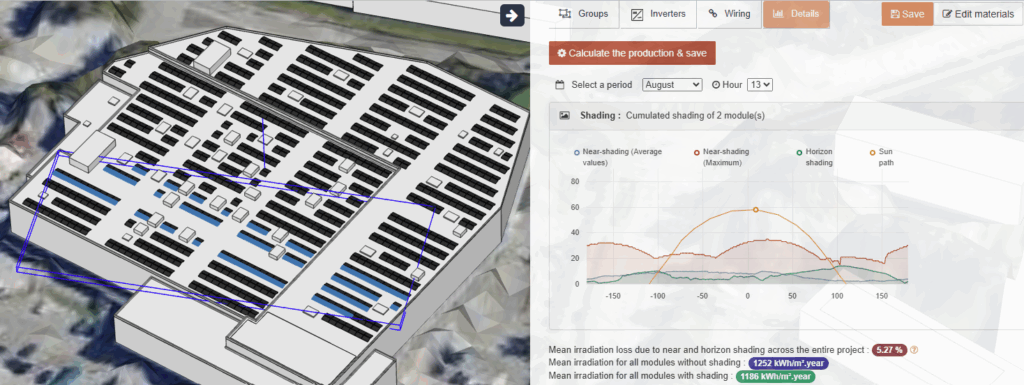
The Distant Mask: Relief and Horizon
Using satellite data (e.g. from NASA), the software calculates the skyline that takes into account the surrounding terrain, such as hills. This relief generates shadows at sunrise and sunset, reducing the available irradiation.
Orientation and inclination
The modules are rarely laid flat: they are oriented and inclined to maximize solar capture. These parameters make it possible to calculate the irradiation actually received in the module plane, while integrating the “IAM” losses.
The Near Mask and 3D Modeling
Shadows created by neighboring buildings, parapets, other rows of modules, or trees may vary from module to module. An advanced simulation is therefore necessarily based on precise 3D modeling in order to evaluate:
- the shadows that are close at all times during the simulation,
- and therefore the differences in sunshine between modules
This approach is essential for complex, heavily shaded installations.

Module performance
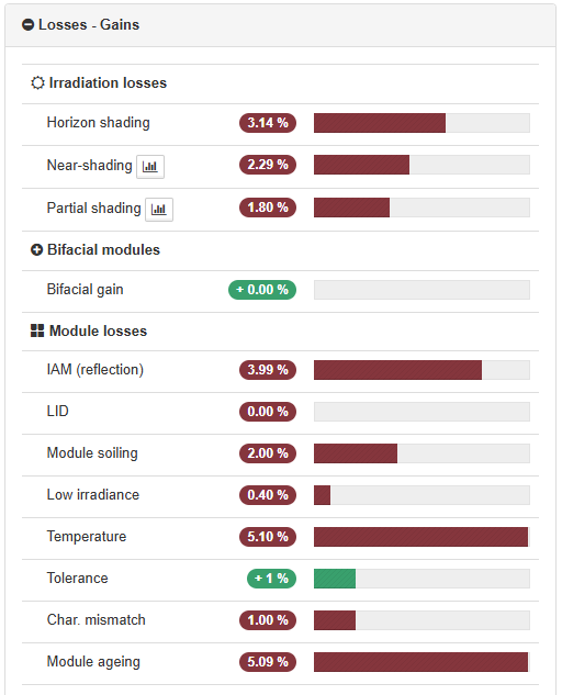
Even when perfectly oriented and inclined, the modules rarely deliver 100% of their nominal power. Several physical phenomena influence their performance.
Module Temperature
Heat reduces the efficiency of photovoltaic panels and is one of the most important sources of losses. The software therefore calculates the actual temperature of the modules based on:
- incident irradiation,
- ambient temperature,
- wind speed,
- rear ventilation.
Fouling
Dust, sand or pollen can cause significant losses. In temperate climates, the impact is usually up to 4%, but it can be much higher depending on the location (quarries, agricultural areas, arid areas).
Low-light losses
The modules react differently depending on the light intensity: their efficiency decreases when the irradiation is low. These variations are incorporated into the simulation.
LID and aging
LID (Light Induced Degradation) occurs from the first hours of sun exposure. In addition, there is a gradual ageing, year after year, which software must also model to simulate production over the entire life of the plant.

Bifaciality: production from the back side
For bifacial modules, part of the production comes from light reflected from the ground or surrounding surfaces, depending on their albedo. The simulation must include:
- a model of the irradiation received by the back side,
- the heterogeneity of this illumination (factor of mismatch losses)
- partial light transmission between cells, modules and module tables.
The quality of this modeling is essential to correctly size bifacial installations and accurately measure their production. Improved accuracy allows for reliable comparison of the sizing variables that have the greatest impact on bifacial gain, such as inclination, height of modules from the ground or roof, distance between rows of modules, etc.
Electrical architecture
Losses in cables
In both direct current (DC) and alternating current (AC), losses in cables are inevitable. When the exact lengths are not yet known, loss values under the nominal conditions, often taken from the standards, are to be used (generally 1%). Losses under actual operating conditions are then calculated.
The performance of the inverter
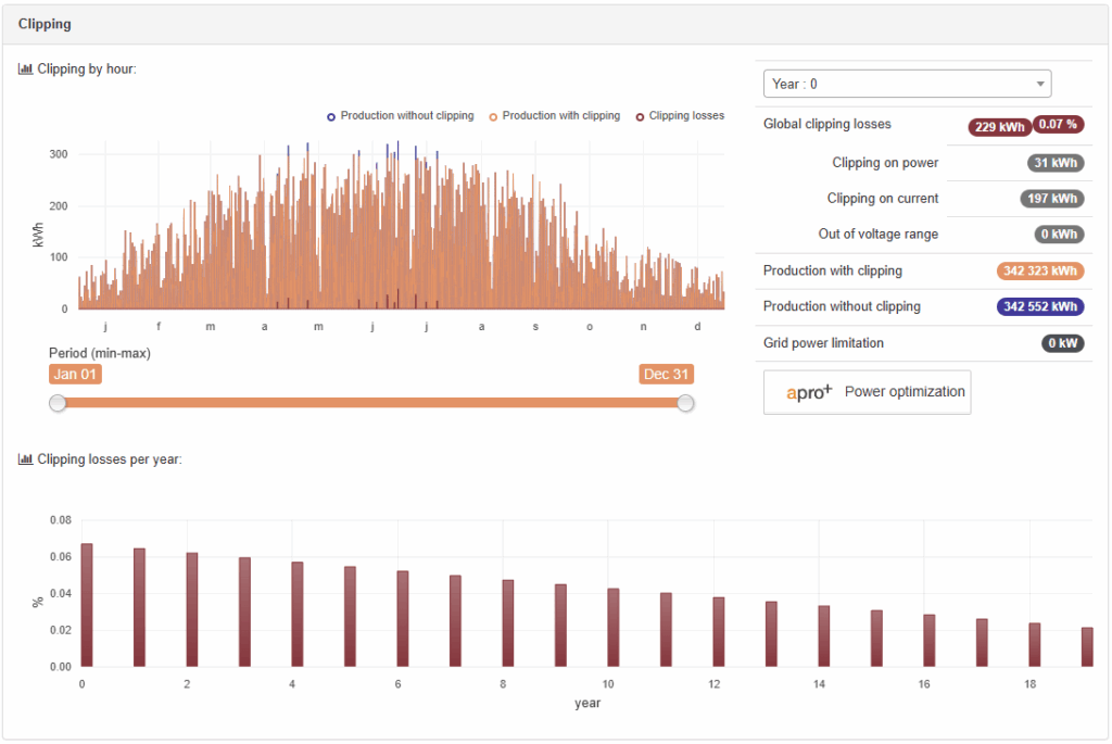
The inverter is one of the most critical components for managing PV module strings, and converting direct current (DC) generation to alternating current (AC) for on-site consumption or grid feed. It must be sized to properly manage the current and voltage of the installation, with correct management of the module chains, possibly distributed over different exposures. The software simulates:
- DC/AC conversion efficiency,
- clipping losses when the DC power exceeds the capacity of the inverter,
- situations outside the voltage or current range,
- the power factor and any reactive power compensation,
- the injection limitations (throttling) that may be imposed by the network operator.
Unavailability and maintenance
Maintenance periods, possible breakdowns or network unavailability also reduce production. These parameters are integrated into the simulation as an unavailability rate.

From physics to statistics: from P50 to P90
Once all the losses have been evaluated, the simulator makes an initial estimate: the P50 output, corresponding to the expected average production. But this average output remains subject to several uncertainties:
- the meteorological data used,
- 3D modeling,
- fouling,
- system availability,
- the actual characteristics of the modules,
- modelling,
These deviations are then integrated into a statistical model usually based on a normal distribution. We thus obtain values:
- P50 which is the average expected production.
- P75 which introduces a moderate risk.
- P90 which corresponds to a conservative production, exceeded in 90% of cases, used to ensure bankability.
These indicators allow investors and banks to assess the financial robustness of the project.

How professional software transforms these complex principles into concrete value
A tool like archelios PRO relies on all these mechanisms to offer a reliable, coherent and justifiable vision of the future production of a photovoltaic power plant. Its added value lies in:
- the reliability of the meteorological databases and the equipment catalogue,
- advanced 3D modeling,
- its ability to produce bankable analyses and reports (P50/P90).
By bringing these elements together, the software makes it possible to move from a simple solar potential to a complete analysis, ready to be presented to an investor, an end customer or a financing organization.
Conclusion: from solar resources to reliable production estimates
The calculation of photovoltaic output is much more than just a theoretical exercise: it is a rigorous process that combines meteorology, physics, thermal, electronics and statistical probability. A powerful simulation application makes it possible to control this complexity and provide a reliable estimate, which is necessary to optimize the design, secure investments and guarantee the sustainability of the project.
Thanks to professional tools like archelios PRO, every PV installation can be accurately simulated, justified and presented with a level of confidence adapted to the requirements of the market.
This article was written by:

Carl WARD
Photovoltaic Product Manager - Trace Software
Carl WARD plays a key role in the development of our archelios range, dedicated to the design and optimisation of photovoltaic projects. "We are passionate about managing these solutions, and thanks to our expertise, we can help professionals to make solar energy more efficient, accessible and sustainable."
